Asperger’s, studying, and writing
As a person with autistic spectrum disorder (ASD), I’ve learned that writing plays an important and meaningful role in my life. I write a lot. By ‘a lot’ I mean to define it as a daily activity. Sometimes I will spend my entire morning and afternoon writing. Other times I will be up through night because my urge to write about something has kept me from sleeping. Most often I write about maths and physics, keeping track of my thoughts and ideas, planning essays, or writing about my work. But I also make it a principle of life to read widely. Indeed, I enjoy reading – studying – as much as I enjoy writing, and this often motivates me to write about many other topics. The two go hand-in-hand.
One reason writing has become important for me has to do with how, as a person with Asperger’s, social communication (by which I mean verbal, but of course also entails other forms like sign) is a source of struggle. I don’t often write about my Asperger’s, mainly because I find it a difficult process. It is hard to organise my thoughts about it, and I am never sure what is appropriate to share. In formal language, my Asperger’s is described clinically as high-functioning but severe. A big part of my life is about learning new strategies to cope. Some of the strategies may even be familiar to others without ASD, like learning to talk in front of others in ways that minimise anxiety and stress, or without completely freaking out (what we call in my language ‘red card’ moments). Or, to give another example, we work on finding strategies for the times I am at the office, so my brain doesn’t go into hyperdrive and so I can focus on discussion and also things like writing on the whiteboard. Another thing about my Asperger’s is that it can be hard adjusting to new people and it can be very stressful acclimatising to new environments. I’ve been working with Tony, now my PhD supervisor, for two years or more and I have only recently started to acclimatise and find our engagement a bit easier to manage. Indeed, in the same time I’ve been at the University of Nottingham, it remains an ongoing process adjusting to this new environment and to being on campus. Like with my close friend, Arnold, who, even after seeing him everyday for years, it was often still a challenge for me to engage with him socially and to visit his house. There is a lot to my experience, not just the social aspect of experience, that can be difficult and demanding as well as overwhelming. I also struggle a lot with anxiety and other things, in addition to extreme sensory sensitivity. So I require a lot of time and space for stillness in my own environment, with my own structure and routine – usually in my own space with my books and other comforts – because sensory overload can easily overwhelm.
In my one attempt to write about living with ASD I expressed how it can be difficult to understand cultural meanings as another example. This is a way of describing orientation to many of the ‘codes’ or behavioural routines that normalise in society. For example, I remember when I was a teenager being pressured a lot to establish the same routine economic patterns as others, or blamed because I didn’t have a job or couldn’t maintain one. I find it difficult to compute things like why daily life is the way it is for most individuals or why people behave as they do. What motivates daily behaviour and routine? How do people make decisions or direct the future course of their lives? Science, textbooks, and studying fervently became, at least in part, a survival-based mechanism. There is no instruction manual about humans; or about why history has taken the path it has in the course of human and societal development; or why many arbitrary social customs have come to be the way they are; or why my father acted and behaved the way he did; among many other things that come to be a feature of life. Studying became my way to cope and to understand, and writing became an extension of that. For instance, I studied every aspect of psychology to help better understand my experiences growing up or why, at least in part, people act violently or use violent language. I’ve read and written across most of philosophy; the same for economics, certainly enough to understand the fundamental debates; and also a lot of sociology. At one point I read a lot of political history, with history one of my favourite subjects. While all of this has a purpose in aiding my attempt to try and understand the world I am a part of, it also supports my passion for studying, my focused interests, and provides the stimulation I need.
On top of it all, living with Asperger’s can be quite exhausting. Indeed, one thing that is common for people diagnosed with autism is the experience of a certain type of fatigue, or what, in my house, we call ‘crashes’. These are a daily experience, where I need to put on my headphones and sit in my own (still and comfortable) space for however long it takes to calm my brain. For these reasons, day to day life is often spent in controlled environments, because it helps ease the red card moments, reducing stress and anxiety, and thus also helps combat the amount of crashes.
I think it all adds up in some sort of complicated sum as to why I find writing an important outlet. But even writing has its own difficulties. I remember my teacher, when I was 6 or 7 years old, say that my brain runs faster than my pen. I think this is true. I think of the sluggish pen effect as the difficulty in converting the internal representations of whatever concept or idea into concise written form at the pace I wish to feed ink to paper. So even though I write everyday and have been practising for many years, the usual result of my writing is typically permeated with errors. The process can be disabling and discouraging, to be honest, with many moments of frustration and failure; but, I’ve also learned that when I battle through and produce something I am happy with, the moment of victory is worth so much.
For many personal reasons, I’ve been regularly encouraged to write more and share more on my blog, and this is something I’ve been working toward. I think that, over a couple of years, I’ve grown more and more comfortable sharing essays and technical notes, although perhaps that is especially true in recent months; but I am also practising writing in other ways, like more personally and less formally. Technical writing is much easier than informal discussion, although a definition of the latter still seems somewhat unclear.
So as one step, this is a new blog post format that I may start experimenting with over the coming weeks, in addition to my usual research entries, essays, and technical notes. Although I prefer to keep my blog focused on my maths and physics research, which of course is mainly string related, allowing from time to time the inclusion of the odd bit of academic diversion, I think this (weekly or fortnightly) format of (n-1)-thoughts may be a fun space that allows me to practice writing in different ways, to share disconnected thoughts or random interests, outside of the formal essay or technical structure.
Generalised geometry, higher structures, and some John Baez papers
Another gem by, Urs! In a recent post on higher structures and M-theory, I made a comment recommending that people read Urs Schreiber’s many notes over the years. In my own research, I’ve found them to be invaluable. The most recent example relates, in some ways, to what I also mentioned in that post about how we may motivate the study of higher structures in fundamental physics: namely, how the Kalb-Ramond 2-form can be seen as an example of a higher structure as it is generalised from the gauge potential 1-form. I won’t go into details here, but the other day I was thinking about such generalisations, and I was thinking about Hamiltonian mechanics in the process. As I’ve mentioned before, if I were to teach string theory one day I would take this approach, emphasising at the outset the important generalisation from point particle theory to the extended object of the string.
Thinking of higher structures, I knew there were many connections here, and I was wanting to fill out my notes, for instance from how in generalised geometry the algebraic structure on  is a Courant Lie 2-algebroid. Those who study DFT will likely be quite familiar with Courant algebroids, and, certainly from a higher structure perspective this line of study is interesting. I also knew there was an original paper, which I had seen in passing, talking about this and the relation to symplectic manifolds, but I couldn’t find it. Then, bam! As Schreiber notes in a forum reply, ‘Courant Lie 2-algebroids (standard or non-standard) play a role in various guises in 2-dimensional QFT, thanks to the fact that they are in a precise sense the next higher analogue of symplectic manifolds and thus the direct generalization of Hamiltonian mechanics from point particles to strings’.
The part ‘from point particles to strings’ was hyperlinked to an important paper, the very paper I was looking for! The paper is Categorified Symplectic Geometry and the Classical String by John C. Baez, Alexander E. Hoffnung, Christopher L. Rogers. I look forward to working through this.
I also want to highlight several other papers from around the same time by Baez, including one co-authored with Schreiber, that I think are also foundational to the programme:
Categorification co-authored with James Dolan;
Higher-Dimensional Algebra VI: Lie 2-Algebras co-authored with Alissa S. Crans;
Lectures on n-Categories and Cohomology co-authored with Michael Shulman;
and, finally, Higher Gauge Theory co-authored with Urs Schreiber.
Thinking about my summer reading list
My summer holiday is in June this year, as I have a conference in mid-July and then I am scheduled to return back to university 1 August. I think Beth and I are going to spend a week in a North Norfolk, one of our favourite places, which has also sort of become a home for both of us. In anticipation of my break, I’ve started putting together my summer reading list, as I do every year. To be honest, there are so many good books right now, it is difficult to choose.
Although my list isn’t complete, one book that I’m already looking forward to is Jennifer Ackerman’s ‘The Genius of Birds‘. I had this book on my Christmas break reading list but, unfortunately, I didn’t have enough time to get to it.
I recently purchased ‘Explaining Humans: What Science Can Teach Us About Life, Love and Relationships’ by Camilla Pang, and I think I will add this to my list. Camilla has a PhD in biochemistry and, as she also has ASD, my interest in this book is more so about her personal journey coming to grips with the complex world social around her through the lens of science. It sounds, on quick glance, that we’ve come to cope with the world in similar ways and share an interest in understanding human behaviour and development. Having said that, I think there is a bit of a risk that people might read this book and conflate it with some sort of autistic worldview, which is completely incorrect, or, equally incorrect, as a scientific view of human behaviour. Contrary to some reviews, I wouldn’t read Pang’s book looking for a strictly scientific view (else one will be disappointed). I could be wrong, but I think ‘Explaining Humans’ may have potentially been mispromoted, hence some of the confused feedback. I approach this book as I would when reading someone’s memoirs, like ‘Diary of a Young Naturalist‘ by Dara McAnulty, ‘Lab girl‘ by Hope Jahren, or ‘Letters to a Young Scientist‘ by Edward O. Wilson. With topics including the challenges of relationships, learning from mistakes, and navigating the human social world by finding tools in things like game theory and machine learning, my interest is in the fact that this is another author with autism and, for myself, I similarly use textbooks and my studies to understand and manage my experience the world. Even on a purely phenomenological level, it will be interesting.
Another book that I may add is of a completely different tone: namely, Saul David’s ‘Crucible of Hell’. I’ve been enjoying reading about WWII again, and, as noted in this post on Dan Carlin’s podcast series on the events in the Asiatic-Pacific theatre, the battle of Okinawa (and others) I haven’t read much about. A few more books I have been thinking about: Douglas R. Hofstadter’s ‘Gödel, Escher, Bach: an Eternal Golden Braid‘, ‘The Deeper Genome‘ by John Parrington, ‘King of Infinite Space: Donald Coxeter, the Man Who Saved Geometry‘ by Siobhan Roberts, ‘Decoding Schopenhauer’s Metaphysics’ by Bernardo Kastrup, ‘Quantum Computing Since Democritus‘ by Scott Aaronson, Jared Diamond’s ‘Guns, Germs, and Steel: The Fates of Human Society‘, and Daniel Kahneman’s latest ‘Noise: A Flaw in Human Judgement‘. Tough decisions.
Linguistics
I’ve been short on time this week finishing some calculations and working on a paper, prior to receiving my second Covid jab. But the other afternoon I thoroughly enjoyed this article. It’s on the Galilean challenge and its reformulation, wherein discussion unfolds on why there is an emerging distinction between the internalised system of knowledge and the processes that access it.
As alluded a moment ago, a general theory of development has interested me for a long time. For my book published by Springer Nature, a lot of the study and references were originally motivated by this interest. When I last did an extensive read on the topic, there was a lot of progress in developmental models – biology, bio- and neuro-linguistics, child psychology, and so on. The summer when I was writing my book, I had already compiled all of my research and I was running short on time in terms of the writing process (I wrote the book in the span of two weeks). Around the time of my research, if I recall there was discussion in biolinguistics regarding the hypothesis of ‘[t]he fibre tract [as one reason] for the difference in language ability in adults compared to pre-linguistic infants’. I remember noting that interesting ideas were developing, and this is a nice article on that front. What is particularly fascinating, I would say, is how language design appears to maximise computation efficiency, but ‘disregards communicative efficiency‘ [italics mine].
This certainly runs directly counter to common belief, as mentioned in the article, namely the established view that communication is a basic function of language. For a long time, as I understand it, there was belief that there was an experiential component to early language formation; but what current research suggests is that, an experiential component is not fundamental at all. Of course an experiential component plays a role, in some capacity, when it comes to externalisation processes, such as in development of variances in regional accent here in England as an example. I mean, the subject is mediated (to whatever degree) by his/her sociohistorical-cultural circumstances, but, unless I am misunderstanding (I need to read through the research more deeply) language itself is not some purely social construct.
Regarding reference to the evolutionary record, I wonder how the developing view in the article relates to ongoing research concerning, for example, certain species of birds, their migratory paths, and the question of inherited or genetic knowledge. It’s an absolutely fascinating area of study, something I’ve been reading about with my interests in mathematical biology, and of course there is very apt analogy here also with broader developments in microbiology.
One last thing of note from reading the article, as I have written quite a bit about the enlightenment philosophes and the start of modern science, it is notable how they sought to ask the question of language. Descartes’ fundamental enquiry into language – the Cartesian question – remains interesting to this day, and I was delighted to see it referenced at the outset. I recommend reading Descartes’ meditations plus other contributions to the enlightenment philosophes – Kant, Spinoza, Hume, to name a few. There is so much here that remains relevant to our modern history and to the development of the contemporary social world. For a few years I’ve been writing a series of essays on Hegel’s science of logic and his epistemology, which is notably relevant today in my area of work in fundamental maths/physics.
Mental health awareness week
Finally, it’s mental health awareness week in the UK. Often these sort of campaigns can be incredibly superficial, failing to look at root causes or ask fundamental questions about well-being and support, but they don’t have to be. Mental health awareness is something that I’ve always taken seriously, not least because I have experienced many challenges with my own mental health throughout my life. The last time I did research and wrote on the subject, suicide statistics in many leading Western countries were significant. I know, too, that for people with autism, like myself, mental health can present a significant challenge in addition to the other challenges one may face. People with autism are much more likely to die by suicide than the general population, as many cause-specific analyses of mortality for people with autistic spectrum disorder (ASD) indicate. Sometimes these facts are overlooked when we talk about mental health as a society, and often I find it important to highlight. But mental health doesn’t discriminate, it affects all people from all backgrounds, and weeks like this one are a good time to help foster discussion, combat stigma, and to think about mental health in all of its facets.
*Image: ‘Streams of Paint‘ by markchadwickart (CC BY-NC-ND 2.0).


 , from which we moved to consider the notion of a generalised tangent bundle such that
  with
with  that preserve the bilinear form is the orthogonal group
  . In the more general case, these endomorphisms become bundle endomorphisms. These bundle endomorphisms are sections of
  . In making this generalisation, the B-transform involves a section of
  , i.e. a two-form. While continuing to preserve the bilinear form, as we’ll see this B-transformation becomes especially important (indeed, another stringy hint resides here).


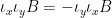


![{[\mathcal{L}_x, \iota_y] = \iota_{[x,y]}}](https://s0.wp.com/latex.php?latex=%7B%5B%5Cmathcal%7BL%7D_x%2C+%5Ciota_y%5D+%3D+%5Ciota_%7B%5Bx%2Cy%5D%7D%7D&bg=ffffff&fg=000000&s=0&c=20201002)


![\displaystyle [e^B X, e^B Y] = e^B [X,Y] - \iota_x \iota_y dB. \ \ \ \ \ (4)](https://s0.wp.com/latex.php?latex=%5Cdisplaystyle++%5Be%5EB+X%2C+e%5EB+Y%5D+%3D+e%5EB+%5BX%2CY%5D+-+%5Ciota_x+%5Ciota_y+dB.+%5C+%5C+%5C+%5C+%5C+%284%29&bg=ffffff&fg=000000&s=0&c=20201002)
![\displaystyle [e^B X, e^B Y] = [e^B (x + \xi), e^B (y + \varepsilon)]](https://s0.wp.com/latex.php?latex=%5Cdisplaystyle+%5Be%5EB+X%2C+e%5EB+Y%5D+%3D+%5Be%5EB+%28x+%2B+%5Cxi%29%2C+e%5EB+%28y+%2B+%5Cvarepsilon%29%5D+&bg=ffffff&fg=000000&s=0&c=20201002)
![\displaystyle = [x + \xi + \iota_x B, y + \varepsilon + \iota_y B]](https://s0.wp.com/latex.php?latex=%5Cdisplaystyle+%3D+%5Bx+%2B+%5Cxi+%2B+%5Ciota_x+B%2C+y+%2B+%5Cvarepsilon+%2B+%5Ciota_y+B%5D+&bg=ffffff&fg=000000&s=0&c=20201002)
![\displaystyle = [x + \xi, y + \varepsilon] + [x, \iota_y B] + [\iota_x B, y]](https://s0.wp.com/latex.php?latex=%5Cdisplaystyle+%3D+%5Bx+%2B+%5Cxi%2C+y+%2B+%5Cvarepsilon%5D+%2B+%5Bx%2C+%5Ciota_y+B%5D+%2B+%5B%5Ciota_x+B%2C+y%5D+&bg=ffffff&fg=000000&s=0&c=20201002)
![\displaystyle = [X,Y] + [x, \iota_y B] +[\iota_x B, y]](https://s0.wp.com/latex.php?latex=%5Cdisplaystyle+%3D+%5BX%2CY%5D+%2B+%5Bx%2C+%5Ciota_y+B%5D+%2B%5B%5Ciota_x+B%2C+y%5D+&bg=ffffff&fg=000000&s=0&c=20201002)
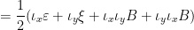
![\displaystyle = [X,Y] + \mathcal{L}_x \iota_y B - \frac{1}{2}d \iota_x \iota_y B - \mathcal{L}_y \iota_x B + \frac{1}{2} d \iota_x \iota_y B](https://s0.wp.com/latex.php?latex=%5Cdisplaystyle+%3D+%5BX%2CY%5D+%2B+%5Cmathcal%7BL%7D_x+%5Ciota_y+B+-+%5Cfrac%7B1%7D%7B2%7Dd+%5Ciota_x+%5Ciota_y+B+-+%5Cmathcal%7BL%7D_y+%5Ciota_x+B+%2B+%5Cfrac%7B1%7D%7B2%7D+d+%5Ciota_x+%5Ciota_y+B+&bg=ffffff&fg=000000&s=0&c=20201002)
![\displaystyle = [X,Y] + (\mathcal{L}_x \iota_y - \mathcal{L}_y \iota_x + d\iota_y \iota_x )B](https://s0.wp.com/latex.php?latex=%5Cdisplaystyle+%3D+%5BX%2CY%5D+%2B+%28%5Cmathcal%7BL%7D_x+%5Ciota_y+-+%5Cmathcal%7BL%7D_y+%5Ciota_x+%2B+d%5Ciota_y+%5Ciota_x+%29B+&bg=ffffff&fg=000000&s=0&c=20201002)
![\displaystyle = [X,Y] + (\mathcal{L}_x \iota_y - \iota_y d\iota_x)B](https://s0.wp.com/latex.php?latex=%5Cdisplaystyle+%3D+%5BX%2CY%5D+%2B+%28%5Cmathcal%7BL%7D_x+%5Ciota_y+-+%5Ciota_y+d%5Ciota_x%29B+&bg=ffffff&fg=000000&s=0&c=20201002)
![\displaystyle = [X,Y] + (\mathcal{L}_x \iota_y - \iota_y d\iota_x)B - \iota_y \iota_x dB + \iota_y \iota_x dB](https://s0.wp.com/latex.php?latex=%5Cdisplaystyle+%3D+%5BX%2CY%5D+%2B+%28%5Cmathcal%7BL%7D_x+%5Ciota_y+-+%5Ciota_y+d%5Ciota_x%29B+-+%5Ciota_y+%5Ciota_x+dB+%2B+%5Ciota_y+%5Ciota_x+dB+&bg=ffffff&fg=000000&s=0&c=20201002)
![\displaystyle = [X,Y] + (\mathcal{L}_x \iota_y - \iota_y \mathcal{L}_x)B + \iota_y \iota_x dB](https://s0.wp.com/latex.php?latex=%5Cdisplaystyle+%3D+%5BX%2CY%5D+%2B+%28%5Cmathcal%7BL%7D_x+%5Ciota_y+-+%5Ciota_y+%5Cmathcal%7BL%7D_x%29B+%2B+%5Ciota_y+%5Ciota_x+dB+&bg=ffffff&fg=000000&s=0&c=20201002)
![\displaystyle = [X,Y] + \iota_{[x,y]}B - \iota_x \iota_y dB](https://s0.wp.com/latex.php?latex=%5Cdisplaystyle+%3D+%5BX%2CY%5D+%2B+%5Ciota_%7B%5Bx%2Cy%5D%7DB+-+%5Ciota_x+%5Ciota_y+dB+&bg=ffffff&fg=000000&s=0&c=20201002)
![\displaystyle = e^B [X,Y] - \iota_x \iota_y dB, \ \ \ \ (5)](https://s0.wp.com/latex.php?latex=%5Cdisplaystyle+%3D+e%5EB+%5BX%2CY%5D+-+%5Ciota_x+%5Ciota_y+dB%2C+%5C+%5C+%5C+%5C+%285%29+&bg=ffffff&fg=000000&s=0&c=20201002)


![{F([A,B]) = [F(A),F(B)] \forall A,B \in \Gamma(TM \oplus T^{\star}M)}](https://s0.wp.com/latex.php?latex=%7BF%28%5BA%2CB%5D%29+%3D+%5BF%28A%29%2CF%28B%29%5D+%5Cforall+A%2CB+%5Cin+%5CGamma%28TM+%5Coplus+T%5E%7B%5Cstar%7DM%29%7D&bg=ffffff&fg=000000&s=0&c=20201002)


![\displaystyle [X,Y]_H = [X,Y]_C + \iota_X \iota_Y H. \ \ \ \ \ (12)](https://s0.wp.com/latex.php?latex=%5Cdisplaystyle+%5BX%2CY%5D_H+%3D+%5BX%2CY%5D_C+%2B+%5Ciota_X+%5Ciota_Y+H.+%5C+%5C+%5C+%5C+%5C+%2812%29&bg=ffffff&fg=000000&s=0&c=20201002)
![\displaystyle [e^B X, e^B Y]_{H -dB} = e^B [X,Y]_H. \ \ \ \ \ (13)](https://s0.wp.com/latex.php?latex=%5Cdisplaystyle+%5Be%5EB+X%2C+e%5EB+Y%5D_%7BH+-dB%7D+%3D+e%5EB+%5BX%2CY%5D_H.+%5C+%5C+%5C+%5C+%5C+%2813%29&bg=ffffff&fg=000000&s=0&c=20201002)


![\displaystyle ([F(x), F(y)]) = F[x,y] \ \forall \ x,y \in \Gamma(TM) \ \ \ \ \ (14)](https://s0.wp.com/latex.php?latex=%5Cdisplaystyle++%28%5BF%28x%29%2C+F%28y%29%5D%29+%3D+F%5Bx%2Cy%5D+%5C+%5Cforall+%5C+x%2Cy+%5Cin+%5CGamma%28TM%29+%5C+%5C+%5C+%5C+%5C+%2814%29&bg=ffffff&fg=000000&s=0&c=20201002)


![\displaystyle [F(X),F(Y)] = F[X,Y] \ \ \ \ \ (15)](https://s0.wp.com/latex.php?latex=%5Cdisplaystyle++%5BF%28X%29%2CF%28Y%29%5D+%3D+F%5BX%2CY%5D+%5C+%5C+%5C+%5C+%5C+%2815%29&bg=ffffff&fg=000000&s=0&c=20201002)


 with
with  a vector space. We can introduce a complex structure on
  satisfying
  . To introduce a symplectic structure on
  such that
  is skew-symmetric
  and non-degenerate (and so
  such that
 ,
,
 ,
,
 is the natural bilinear form on
  defines a generalised complex structure

 denotes the dual map
  .
.


 . After diagonalisation we find

 . In other words, as
  is the constant
  transformations
  such that
  is the property of split orthogonal matrices. (There is no restriction on the vector fields being integers and hence they take values in
  ).
).
 ) In fact, as we have seen in the proceeding analysis, the
  acts on the fibres
  .
.
 . The metric
  , where
  given by
  . Then it can be found
  such that the restriction to the natural form
  to
to  be a positive definite subbundle of rank
  .
.
 , define
  and
and  , which is the orthogonal compliment of
  with the form
  and negative definition on
  . If we switch the sign on
  .
.
 is isotropic,
  . So, similar to the standard Riemannian example, we can write
  where
where  . We can now split
  into symmetric and anti-symmetric parts such that
  with
with
 ,
,
 .
.
 . Since
  is positive definite it follows
  defined as multiplication by
  . Then it can be shown that we have a bilinear form on
  . Then for a tangent vector
  ,
,  so that
  . Similarly
  , which means that in matrix form

 where we define
  as the subbundles when
  where
where  is (
is (
 matrix


 the metric on
  obtained by inverting

 over
over  called the anchor, or anchor map;
![{[ \cdot , \cdot ]}](https://s0.wp.com/latex.php?latex=%7B%5B+%5Ccdot+%2C+%5Ccdot+%5D%7D&bg=ffffff&fg=000000&s=0&c=20201002) , on smooth sections
, on smooth sections  satisfying a Lie algebra
 is a Lie algebra homomorphism and the following relations are satisfied
![\displaystyle \pi ([X,Y]) = [\pi (X), \pi (Y)],](https://s0.wp.com/latex.php?latex=%5Cdisplaystyle++%5Cpi+%28%5BX%2CY%5D%29+%3D+%5B%5Cpi+%28X%29%2C+%5Cpi+%28Y%29%5D%2C+&bg=ffffff&fg=000000&s=0&c=20201002)
![\displaystyle \ [X, fY] = f[X,Y] + (\pi (X)f)Y, \ \ \ \ \ (1)](https://s0.wp.com/latex.php?latex=%5Cdisplaystyle++%5C+%5BX%2C+fY%5D+%3D+f%5BX%2CY%5D+%2B+%28%5Cpi+%28X%29f%29Y%2C+%5C+%5C+%5C+%5C+%5C+%281%29&bg=ffffff&fg=000000&s=0&c=20201002)
 and
and  . In this case, the first condition in (
![{(TM \oplus T^{\star}M, [\cdot, \cdot])}](https://s0.wp.com/latex.php?latex=%7B%28TM+%5Coplus+T%5E%7B%5Cstar%7DM%2C+%5B%5Ccdot%2C+%5Ccdot%5D%29%7D&bg=ffffff&fg=000000&s=0&c=20201002) we don’t have a Lie algebroid.
we don’t have a Lie algebroid.
 , which is involutive (i.e., self-inverse is its own inverse) such that it is isotropic and closed under the Courant bracket. Then the inner products in the Nijenhuis operator vanish, meaning
 ![{(N, [\cdot, \cdot], \pi)}](https://s0.wp.com/latex.php?latex=%7B%28N%2C+%5B%5Ccdot%2C+%5Ccdot%5D%2C+%5Cpi%29%7D&bg=ffffff&fg=000000&s=0&c=20201002) would be a Lie algebroid. It can also be proven now that the second condition is also satisfied.
would be a Lie algebroid. It can also be proven now that the second condition is also satisfied.
 be a subbundle of
  for all
  . Given that the inner product has signature
  , the maximal dimensions of the subspace is
  . In the case that the dimension of the subspace is
  , which is an example of a complex Lie algebroid.
 , where
  is a subbundle of
  . Then, given an open cover
  of
of  such that on
  , we can say
  describing a 0-cocycle in
  . The next object in the hierarchy is a
  line bundle. This is simply a 1-cocycle
  . It follows that for some
  the third object in the hierarchy is a gerbe, which is a 2-cocycle in
  . This is a collection of
  .
One then defines a connection on the gerbe as a collection of one-forms
.
One then defines a connection on the gerbe as a collection of one-forms  defined on the double intersections with
  . On triple intersections the connection satisfies


 on the
  such that on double intersections

 with connection
  . Then, over each
  the fibres are related by a B-transform

 such that on double intersections the relation
  is satisfied.
 . These 2-forms yield an isomorphism
  which over
  . Locally, the isomorphism
  is a B-transform. Define this B-transform by
![\displaystyle [\phi(X), \phi(Y)]= \phi([X,Y]) - \iota_x \iota_y dB_a = \phi([X,Y]) - \iota_x \iota_y H, \ \ \ \ (7)](https://s0.wp.com/latex.php?latex=%5Cdisplaystyle+%5B%5Cphi%28X%29%2C+%5Cphi%28Y%29%5D%3D+%5Cphi%28%5BX%2CY%5D%29+-+%5Ciota_x+%5Ciota_y+dB_a+%3D+%5Cphi%28%5BX%2CY%5D%29+-+%5Ciota_x+%5Ciota_y+H%2C+%5C+%5C+%5C+%5C+%287%29&bg=ffffff&fg=000000&s=0&c=20201002)
 over
over  with
with ![{[ \ , ]}](https://s0.wp.com/latex.php?latex=%7B%5B+%5C+%2C+%5D%7D&bg=ffffff&fg=000000&s=0&c=20201002) on the twisted generalised tangent bundle
on the twisted generalised tangent bundle ![\displaystyle [X,Y]_H = [X,Y] - \iota_x \iota_y H, \ \ \ \ \ (8)](https://s0.wp.com/latex.php?latex=%5Cdisplaystyle++%5BX%2CY%5D_H+%3D+%5BX%2CY%5D+-+%5Ciota_x+%5Ciota_y+H%2C+%5C+%5C+%5C+%5C+%5C+%288%29&bg=ffffff&fg=000000&s=0&c=20201002)
![\displaystyle [\phi(X), \phi(Y)] = \phi[X,Y]_H \ \ \ (9)](https://s0.wp.com/latex.php?latex=%5Cdisplaystyle+%5B%5Cphi%28X%29%2C+%5Cphi%28Y%29%5D+%3D+%5Cphi%5BX%2CY%5D_H+%5C+%5C+%5C+%289%29&bg=ffffff&fg=000000&s=0&c=20201002)
![\displaystyle [e^B X, e^B Y]_H = e^B [X,Y]_{H + dB}. \ \ \ (10)](https://s0.wp.com/latex.php?latex=%5Cdisplaystyle+%5Be%5EB+X%2C+e%5EB+Y%5D_H+%3D+e%5EB+%5BX%2CY%5D_%7BH+%2B+dB%7D.+%5C+%5C+%5C+%2810%29&bg=ffffff&fg=000000&s=0&c=20201002)
![\displaystyle \mathcal{L}_X = d\iota_X + \iota_X d, \ \iota_{[X,Y]} = [\mathcal{L}_X, \iota_Y]. \ \ \ \ \ (1)](https://s0.wp.com/latex.php?latex=%5Cdisplaystyle++%5Cmathcal%7BL%7D_X+%3D+d%5Ciota_X+%2B+%5Ciota_X+d%2C+%5C+%5Ciota_%7B%5BX%2CY%5D%7D+%3D+%5B%5Cmathcal%7BL%7D_X%2C+%5Ciota_Y%5D.+%5C+%5C+%5C+%5C+%5C+%281%29&bg=ffffff&fg=000000&s=0&c=20201002)
![\displaystyle \iota_{[X,Y]} = d\iota_X \iota_Y + \iota_X d\iota_Y - \iota_Y d\iota_X - \iota_Y \iota_X d, \ \ \ \ \ (2)](https://s0.wp.com/latex.php?latex=%5Cdisplaystyle++%5Ciota_%7B%5BX%2CY%5D%7D+%3D+d%5Ciota_X+%5Ciota_Y+%2B+%5Ciota_X+d%5Ciota_Y+-+%5Ciota_Y+d%5Ciota_X+-+%5Ciota_Y+%5Ciota_X+d%2C+%5C+%5C+%5C+%5C+%5C+%282%29&bg=ffffff&fg=000000&s=0&c=20201002)


![\displaystyle [x + \xi, y + \varepsilon] \cdot \omega = [\mathcal{L}_{x + \xi}, (y + \varepsilon)] \cdot \omega](https://s0.wp.com/latex.php?latex=%5Cdisplaystyle++%5Bx+%2B+%5Cxi%2C+y+%2B+%5Cvarepsilon%5D+%5Ccdot+%5Comega+%3D+%5B%5Cmathcal%7BL%7D_%7Bx+%2B+%5Cxi%7D%2C+%28y+%2B+%5Cvarepsilon%29%5D+%5Ccdot+%5Comega+&bg=ffffff&fg=000000&s=0&c=20201002)

![\displaystyle = \iota_{[x,y]} \omega + \mathcal{L}_x (\varepsilon \wedge \omega) - \varepsilon \wedge \mathcal{L}_x \omega + d\xi \wedge \iota_y \omega - \iota_y (d\xi \wedge \omega)](https://s0.wp.com/latex.php?latex=%5Cdisplaystyle++%3D+%5Ciota_%7B%5Bx%2Cy%5D%7D+%5Comega+%2B+%5Cmathcal%7BL%7D_x+%28%5Cvarepsilon+%5Cwedge+%5Comega%29+-+%5Cvarepsilon+%5Cwedge+%5Cmathcal%7BL%7D_x+%5Comega+%2B+d%5Cxi+%5Cwedge+%5Ciota_y+%5Comega+-+%5Ciota_y+%28d%5Cxi+%5Cwedge+%5Comega%29+&bg=ffffff&fg=000000&s=0&c=20201002)
![\displaystyle = \iota_{[x,y]}\omega + \mathcal{L}_x (\varepsilon) \wedge \omega - \iota_y d\xi \wedge \omega. \ \ \ \ \ (4)](https://s0.wp.com/latex.php?latex=%5Cdisplaystyle++%3D+%5Ciota_%7B%5Bx%2Cy%5D%7D%5Comega+%2B+%5Cmathcal%7BL%7D_x+%28%5Cvarepsilon%29+%5Cwedge+%5Comega+-+%5Ciota_y+d%5Cxi+%5Cwedge+%5Comega.+%5C+%5C+%5C+%5C+%5C+%284%29&bg=ffffff&fg=000000&s=0&c=20201002)
 . Its origin comes from the study of Dirac structures, taking the general form
![\displaystyle X \circ Y = (x + \xi) \circ (y + \varepsilon) = [x,y] + \mathcal{L}_x \varepsilon - \iota_y d\xi, \ \ \ \ \ (5)](https://s0.wp.com/latex.php?latex=%5Cdisplaystyle++X+%5Ccirc+Y+%3D+%28x+%2B+%5Cxi%29+%5Ccirc+%28y+%2B+%5Cvarepsilon%29+%3D+%5Bx%2Cy%5D+%2B+%5Cmathcal%7BL%7D_x+%5Cvarepsilon+-+%5Ciota_y+d%5Cxi%2C+%5C+%5C+%5C+%5C+%5C+%285%29&bg=ffffff&fg=000000&s=0&c=20201002)

![{[X,Y] = \frac{1}{2}[X,Y]_D - \frac{1}{2}[Y,X]_D}](https://s0.wp.com/latex.php?latex=%7B%5BX%2CY%5D+%3D+%5Cfrac%7B1%7D%7B2%7D%5BX%2CY%5D_D+-+%5Cfrac%7B1%7D%7B2%7D%5BY%2CX%5D_D%7D&bg=ffffff&fg=000000&s=0&c=20201002) is the Courant bracket.
is the Courant bracket.
 on
on ![\displaystyle [X,Y]_C = [x + \xi, y + \varepsilon]_C = [x,y]_L + \mathcal{L}_x \varepsilon - \mathcal{L}_y \xi - \frac{1}{2} d(\iota_x \varepsilon - \iota_y \xi), \ \ \ \ \ (8)](https://s0.wp.com/latex.php?latex=%5Cdisplaystyle++%5BX%2CY%5D_C+%3D+%5Bx+%2B+%5Cxi%2C+y+%2B+%5Cvarepsilon%5D_C+%3D+%5Bx%2Cy%5D_L+%2B+%5Cmathcal%7BL%7D_x+%5Cvarepsilon+-+%5Cmathcal%7BL%7D_y+%5Cxi+-+%5Cfrac%7B1%7D%7B2%7D+d%28%5Ciota_x+%5Cvarepsilon+-+%5Ciota_y+%5Cxi%29%2C+%5C+%5C+%5C+%5C+%5C+%288%29&bg=ffffff&fg=000000&s=0&c=20201002)
![{[x,y]_L}](https://s0.wp.com/latex.php?latex=%7B%5Bx%2Cy%5D_L%7D&bg=ffffff&fg=000000&s=0&c=20201002) denotes the usual Lie bracket of vector fields and
denotes the usual Lie bracket of vector fields and  denotes contraction with the vector field
  .
.
 satisfy the following relations:
![\displaystyle \mathcal{L}_x = d\iota_x + \iota_x d, \ \mathcal{L}_{[x,y]_L} = [\mathcal{L}_x, \mathcal{L}_y], \ \iota_{[x,y]_L} = [\mathcal{L}_x, \iota_y]. \ \ \ \ \ (9)](https://s0.wp.com/latex.php?latex=%5Cdisplaystyle++%5Cmathcal%7BL%7D_x+%3D+d%5Ciota_x+%2B+%5Ciota_x+d%2C+%5C+%5Cmathcal%7BL%7D_%7B%5Bx%2Cy%5D_L%7D+%3D+%5B%5Cmathcal%7BL%7D_x%2C+%5Cmathcal%7BL%7D_y%5D%2C+%5C+%5Ciota_%7B%5Bx%2Cy%5D_L%7D+%3D+%5B%5Cmathcal%7BL%7D_x%2C+%5Ciota_y%5D.+%5C+%5C+%5C+%5C+%5C+%289%29&bg=ffffff&fg=000000&s=0&c=20201002)
![\displaystyle [X,Y] = [X,Y]_D - d(Y,X), \ \ (10)](https://s0.wp.com/latex.php?latex=%5Cdisplaystyle+%5BX%2CY%5D+%3D+%5BX%2CY%5D_D+-+d%28Y%2CX%29%2C+%5C+%5C+%2810%29+&bg=ffffff&fg=000000&s=0&c=20201002)
![\displaystyle [X,Y]_D + [Y,X]_D = \mathcal{L}_x \varepsilon + \mathcal{L}_y \xi -\iota_x d\varepsilon - \iota_y d\xi = d(\iota_x d\varepsilon + \iota_y \xi) = 2d(X,Y). \ \ (11)](https://s0.wp.com/latex.php?latex=%5Cdisplaystyle+%5BX%2CY%5D_D+%2B+%5BY%2CX%5D_D+%3D+%5Cmathcal%7BL%7D_x+%5Cvarepsilon+%2B+%5Cmathcal%7BL%7D_y+%5Cxi+-%5Ciota_x+d%5Cvarepsilon+-+%5Ciota_y+d%5Cxi+%3D+d%28%5Ciota_x+d%5Cvarepsilon+%2B+%5Ciota_y+%5Cxi%29+%3D+2d%28X%2CY%29.+%5C+%5C+%2811%29+&bg=ffffff&fg=000000&s=0&c=20201002)
![{[X,Y]_D = [X,Y]}](https://s0.wp.com/latex.php?latex=%7B%5BX%2CY%5D_D+%3D+%5BX%2CY%5D%7D&bg=ffffff&fg=000000&s=0&c=20201002) . If we define the projection
. If we define the projection  onto the first factor it follows
![\displaystyle \pi ([X,Y]_D) = [\pi(X),\pi(Y)], \ \ \ \ \ (12)](https://s0.wp.com/latex.php?latex=%5Cdisplaystyle++%5Cpi+%28%5BX%2CY%5D_D%29+%3D+%5B%5Cpi%28X%29%2C%5Cpi%28Y%29%5D%2C+%5C+%5C+%5C+%5C+%5C+%2812%29&bg=ffffff&fg=000000&s=0&c=20201002)
![\displaystyle \pi ([X,Y]) = [\pi X, \pi Y]. \ \ \ \ \ (13)](https://s0.wp.com/latex.php?latex=%5Cdisplaystyle++%5Cpi+%28%5BX%2CY%5D%29+%3D+%5B%5Cpi+X%2C+%5Cpi+Y%5D.+%5C+%5C+%5C+%5C+%5C+%2813%29&bg=ffffff&fg=000000&s=0&c=20201002)
 of
of ![\displaystyle \pi (X) (Y,Z) = ([X,Y]_D, Z) + (X, [Y,Z]_D). \ \ \ \ \ (14)](https://s0.wp.com/latex.php?latex=%5Cdisplaystyle++%5Cpi+%28X%29+%28Y%2CZ%29+%3D+%28%5BX%2CY%5D_D%2C+Z%29+%2B+%28X%2C+%5BY%2CZ%5D_D%29.+%5C+%5C+%5C+%5C+%5C+%2814%29&bg=ffffff&fg=000000&s=0&c=20201002)
 . Start with the right-hand side
![\displaystyle ([x,y] + \mathcal{L}_x \varepsilon - \iota_y d\xi, z + \zeta) + (y + \varepsilon, [x,z] + \mathcal{L}_x \zeta - \iota_z d\xi)](https://s0.wp.com/latex.php?latex=%5Cdisplaystyle++%28%5Bx%2Cy%5D+%2B+%5Cmathcal%7BL%7D_x+%5Cvarepsilon+-+%5Ciota_y+d%5Cxi%2C+z+%2B+%5Czeta%29+%2B+%28y+%2B+%5Cvarepsilon%2C+%5Bx%2Cz%5D+%2B+%5Cmathcal%7BL%7D_x+%5Czeta+-+%5Ciota_z+d%5Cxi%29+&bg=ffffff&fg=000000&s=0&c=20201002)
![\displaystyle = \frac{1}{2}(\iota_{[x,y]} \zeta + \iota_z (\mathcal{L}_x \varepsilon - \iota_y d\xi) + \iota_{[x,z]} \varepsilon + \iota_y (\mathcal{L}_x \zeta - \iota_z d\xi))](https://s0.wp.com/latex.php?latex=%5Cdisplaystyle++%3D+%5Cfrac%7B1%7D%7B2%7D%28%5Ciota_%7B%5Bx%2Cy%5D%7D+%5Czeta+%2B+%5Ciota_z+%28%5Cmathcal%7BL%7D_x+%5Cvarepsilon+-+%5Ciota_y+d%5Cxi%29+%2B+%5Ciota_%7B%5Bx%2Cz%5D%7D+%5Cvarepsilon+%2B+%5Ciota_y+%28%5Cmathcal%7BL%7D_x+%5Czeta+-+%5Ciota_z+d%5Cxi%29%29+&bg=ffffff&fg=000000&s=0&c=20201002)
![\displaystyle = \frac{1}{2} ([\mathcal{L}_{\xi}, \iota_y]\zeta + \iota_z \mathcal{L}_x \varepsilon + [\mathcal{L}_x, \iota_z] \varepsilon + \iota_y \mathcal{L}_x \zeta)](https://s0.wp.com/latex.php?latex=%5Cdisplaystyle++%3D+%5Cfrac%7B1%7D%7B2%7D+%28%5B%5Cmathcal%7BL%7D_%7B%5Cxi%7D%2C+%5Ciota_y%5D%5Czeta+%2B+%5Ciota_z+%5Cmathcal%7BL%7D_x+%5Cvarepsilon+%2B+%5B%5Cmathcal%7BL%7D_x%2C+%5Ciota_z%5D+%5Cvarepsilon+%2B+%5Ciota_y+%5Cmathcal%7BL%7D_x+%5Czeta%29+&bg=ffffff&fg=000000&s=0&c=20201002)


![\displaystyle \pi(X)(Y,Z) = ([X,Y] + d[X,Y], Z) + (Y, [X,Z] + d(X,Z)), \ \ \ \ \ (16)](https://s0.wp.com/latex.php?latex=%5Cdisplaystyle++%5Cpi%28X%29%28Y%2CZ%29+%3D+%28%5BX%2CY%5D+%2B+d%5BX%2CY%5D%2C+Z%29+%2B+%28Y%2C+%5BX%2CZ%5D+%2B+d%28X%2CZ%29%29%2C+%5C+%5C+%5C+%5C+%5C+%2816%29&bg=ffffff&fg=000000&s=0&c=20201002)
![\displaystyle [X, fY]_D = f[X,Y]_D + (\pi (X)f)Y \ \ \ \ \ (17)](https://s0.wp.com/latex.php?latex=%5Cdisplaystyle+%5BX%2C+fY%5D_D+%3D+f%5BX%2CY%5D_D+%2B+%28%5Cpi+%28X%29f%29Y+%5C+%5C+%5C+%5C+%5C+%2817%29&bg=ffffff&fg=000000&s=0&c=20201002)
![\displaystyle [fY, X]_D = f[Y,X]_D + (\pi (X)f)Y - 2 (X,Y)df. \ \ \ \ \ (18)](https://s0.wp.com/latex.php?latex=%5Cdisplaystyle+%5BfY%2C+X%5D_D+%3D+f%5BY%2CX%5D_D+%2B+%28%5Cpi+%28X%29f%29Y+-+2+%28X%2CY%29df.+%5C+%5C+%5C+%5C+%5C+%2818%29&bg=ffffff&fg=000000&s=0&c=20201002)
![\displaystyle [X, fY]_C = f[X,Y] + (\pi (X)f)Y - (X,Y)df. \ \ \ \ \ (19)](https://s0.wp.com/latex.php?latex=%5Cdisplaystyle++%5BX%2C+fY%5D_C+%3D+f%5BX%2CY%5D+%2B+%28%5Cpi+%28X%29f%29Y+-+%28X%2CY%29df.+%5C+%5C+%5C+%5C+%5C+%2819%29&bg=ffffff&fg=000000&s=0&c=20201002)
 , then the Jacobiator can be written as
![\displaystyle Jac(X,Y,Z) = [[X,Y],Z] + [[Y,Z],X] + [[Z,X],Y]. \ \ \ \ \ (20)](https://s0.wp.com/latex.php?latex=%5Cdisplaystyle++Jac%28X%2CY%2CZ%29+%3D+%5B%5BX%2CY%5D%2CZ%5D+%2B+%5B%5BY%2CZ%5D%2CX%5D+%2B+%5B%5BZ%2CX%5D%2CY%5D.+%5C+%5C+%5C+%5C+%5C+%2820%29&bg=ffffff&fg=000000&s=0&c=20201002)
![\displaystyle [X, [Y,Z]_D]_D = [[X,Y]_D , Z]_D + [Y, [X,Z]_D ]_D, \ \ \ \ \ (21)](https://s0.wp.com/latex.php?latex=%5Cdisplaystyle++%5BX%2C+%5BY%2CZ%5D_D%5D_D+%3D+%5B%5BX%2CY%5D_D+%2C+Z%5D_D+%2B+%5BY%2C+%5BX%2CZ%5D_D+%5D_D%2C+%5C+%5C+%5C+%5C+%5C+%2821%29&bg=ffffff&fg=000000&s=0&c=20201002)
![{[X, \ ]_D}](https://s0.wp.com/latex.php?latex=%7B%5BX%2C+%5C+%5D_D%7D&bg=ffffff&fg=000000&s=0&c=20201002) acts as a derivative of the Dorfman bracket. If the Dorfman bracket was skew-symmetric, then this would be equivalent to the Jacobi identity.
acts as a derivative of the Dorfman bracket. If the Dorfman bracket was skew-symmetric, then this would be equivalent to the Jacobi identity.![\displaystyle [[X,Y]_D , Z]_D + [Y, [X,Z]_D ]_D](https://s0.wp.com/latex.php?latex=%5Cdisplaystyle+%5B%5BX%2CY%5D_D+%2C+Z%5D_D+%2B+%5BY%2C+%5BX%2CZ%5D_D+%5D_D+&bg=ffffff&fg=000000&s=0&c=20201002)
![\displaystyle = [[x,y] + \mathcal{L}_x \varepsilon - \iota_y d\xi, z + \zeta] + [y + \varepsilon, [x,z] + \mathcal{L}x \zeta - \iota_z d\xi](https://s0.wp.com/latex.php?latex=%5Cdisplaystyle+%3D+%5B%5Bx%2Cy%5D+%2B+%5Cmathcal%7BL%7D_x+%5Cvarepsilon+-+%5Ciota_y+d%5Cxi%2C+z+%2B+%5Czeta%5D+%2B+%5By+%2B+%5Cvarepsilon%2C+%5Bx%2Cz%5D+%2B+%5Cmathcal%7BL%7Dx+%5Czeta+-+%5Ciota_z+d%5Cxi+&bg=ffffff&fg=000000&s=0&c=20201002)
![\displaystyle = [[x,y], z] + [y, [x,z]] + \mathcal{L}_{[x,y]} \zeta - \iota_z d (\mathcal{L}_x \varepsilon - \iota_y d\xi) + \mathcal{L}_y (\mathcal{L}_x \zeta - \iota_z d\xi ) - \iota_{[x,z]} d\varepsilon](https://s0.wp.com/latex.php?latex=%5Cdisplaystyle+%3D+%5B%5Bx%2Cy%5D%2C+z%5D+%2B+%5By%2C+%5Bx%2Cz%5D%5D+%2B+%5Cmathcal%7BL%7D_%7B%5Bx%2Cy%5D%7D+%5Czeta+-+%5Ciota_z+d+%28%5Cmathcal%7BL%7D_x+%5Cvarepsilon+-+%5Ciota_y+d%5Cxi%29+%2B+%5Cmathcal%7BL%7D_y+%28%5Cmathcal%7BL%7D_x+%5Czeta+-+%5Ciota_z+d%5Cxi+%29+-+%5Ciota_%7B%5Bx%2Cz%5D%7D+d%5Cvarepsilon+&bg=ffffff&fg=000000&s=0&c=20201002)
![\displaystyle = [x, [y,z]] + \mathcal{L}_x \mathcal{L}_y \zeta - \mathcal{L}_y \mathcal{L}_x \zeta - \iota_z \mathcal{L}_x d\varepsilon - \iota_z \mathcal{L}_y d\xi + \mathcal{L}_y \mathcal{L}_x \zeta - \mathcal{L}_y \iota_z d\xi - \iota_{[x,z]} d\varepsilon](https://s0.wp.com/latex.php?latex=%5Cdisplaystyle+%3D+%5Bx%2C+%5By%2Cz%5D%5D+%2B+%5Cmathcal%7BL%7D_x+%5Cmathcal%7BL%7D_y+%5Czeta+-+%5Cmathcal%7BL%7D_y+%5Cmathcal%7BL%7D_x+%5Czeta+-+%5Ciota_z+%5Cmathcal%7BL%7D_x+d%5Cvarepsilon+-+%5Ciota_z+%5Cmathcal%7BL%7D_y+d%5Cxi+%2B+%5Cmathcal%7BL%7D_y+%5Cmathcal%7BL%7D_x+%5Czeta+-+%5Cmathcal%7BL%7D_y+%5Ciota_z+d%5Cxi+-+%5Ciota_%7B%5Bx%2Cz%5D%7D+d%5Cvarepsilon+&bg=ffffff&fg=000000&s=0&c=20201002)
![\displaystyle = [x,[y,z]] + \mathcal{L}_x \mathcal{L}_y \zeta - \iota_{[y,z]}d\xi - \mathcal{L}_x \iota_z d \varepsilon](https://s0.wp.com/latex.php?latex=%5Cdisplaystyle+%3D+%5Bx%2C%5By%2Cz%5D%5D+%2B+%5Cmathcal%7BL%7D_x+%5Cmathcal%7BL%7D_y+%5Czeta+-+%5Ciota_%7B%5By%2Cz%5D%7Dd%5Cxi+-+%5Cmathcal%7BL%7D_x+%5Ciota_z+d+%5Cvarepsilon+&bg=ffffff&fg=000000&s=0&c=20201002)
![\displaystyle = [x,[y,z]] + \mathcal{L}_x (\mathcal{L}_y \zeta - \iota_z d\varepsilon) - \iota_{[y,z]}d\xi](https://s0.wp.com/latex.php?latex=%5Cdisplaystyle+%3D+%5Bx%2C%5By%2Cz%5D%5D+%2B+%5Cmathcal%7BL%7D_x+%28%5Cmathcal%7BL%7D_y+%5Czeta+-+%5Ciota_z+d%5Cvarepsilon%29+-+%5Ciota_%7B%5By%2Cz%5D%7Dd%5Cxi+&bg=ffffff&fg=000000&s=0&c=20201002)
![\displaystyle = [X, [Y,Z]_D]_D. \ \ \ \ \ (22)](https://s0.wp.com/latex.php?latex=%5Cdisplaystyle+%3D+%5BX%2C+%5BY%2CZ%5D_D%5D_D.+%5C+%5C+%5C+%5C+%5C+%2822%29+&bg=ffffff&fg=000000&s=0&c=20201002)
![{[[X,Y]_D , Z]_D}](https://s0.wp.com/latex.php?latex=%7B%5B%5BX%2CY%5D_D+%2C+Z%5D_D%7D&bg=ffffff&fg=000000&s=0&c=20201002) to
to ![{[[X,Y],Z]}](https://s0.wp.com/latex.php?latex=%7B%5B%5BX%2CY%5D%2CZ%5D%7D&bg=ffffff&fg=000000&s=0&c=20201002) such that
such that
![\displaystyle [[X,Y]_D , Z]_D = [[X,Y] + d(X,Y), Z]_D](https://s0.wp.com/latex.php?latex=%5Cdisplaystyle++%5B%5BX%2CY%5D_D+%2C+Z%5D_D+%3D+%5B%5BX%2CY%5D+%2B+d%28X%2CY%29%2C+Z%5D_D+&bg=ffffff&fg=000000&s=0&c=20201002)
![\displaystyle = [[X,Y], Z]_D](https://s0.wp.com/latex.php?latex=%5Cdisplaystyle++%3D+%5B%5BX%2CY%5D%2C+Z%5D_D+&bg=ffffff&fg=000000&s=0&c=20201002)
![\displaystyle = [[X,Y], Z] + d([X,Y],Z), \ \ \ \ \ (23)](https://s0.wp.com/latex.php?latex=%5Cdisplaystyle++%3D+%5B%5BX%2CY%5D%2C+Z%5D+%2B+d%28%5BX%2CY%5D%2CZ%29%2C+%5C+%5C+%5C+%5C+%5C+%2823%29&bg=ffffff&fg=000000&s=0&c=20201002)
![{[a,b]_D = 0}](https://s0.wp.com/latex.php?latex=%7B%5Ba%2Cb%5D_D+%3D+0%7D&bg=ffffff&fg=000000&s=0&c=20201002) when
when  is a closed one-form.
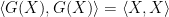
![\displaystyle Nij(X,Y,Z) = \frac{1}{3} (\langle [X,Y],Z \rangle + \langle [Y,Z], X \rangle + \langle [Z,X], Y \rangle, \ \ \ \ \ (25)](https://s0.wp.com/latex.php?latex=%5Cdisplaystyle++Nij%28X%2CY%2CZ%29+%3D+%5Cfrac%7B1%7D%7B3%7D+%28%5Clangle+%5BX%2CY%5D%2CZ+%5Crangle+%2B+%5Clangle+%5BY%2CZ%5D%2C+X+%5Crangle+%2B+%5Clangle+%5BZ%2CX%5D%2C+Y+%5Crangle%2C+%5C+%5C+%5C+%5C+%5C+%2825%29&bg=ffffff&fg=000000&s=0&c=20201002)
![\displaystyle Jac(X,Y,Z) = [[X,Y],Z] + \text{cyclic permutations}](https://s0.wp.com/latex.php?latex=%5Cdisplaystyle+Jac%28X%2CY%2CZ%29+%3D+%5B%5BX%2CY%5D%2CZ%5D+%2B++%5Ctext%7Bcyclic+permutations%7D+&bg=ffffff&fg=000000&s=0&c=20201002)
![\displaystyle = \frac{1}{4} ([[X,Y]_D, Z]_D - [[Y,X]_D, Z]_D - [Z, [X,Y]_D]_D + [Z, [Y,Z]_D]_D + \text{cyclic permutations}](https://s0.wp.com/latex.php?latex=%5Cdisplaystyle+%3D+%5Cfrac%7B1%7D%7B4%7D+%28%5B%5BX%2CY%5D_D%2C+Z%5D_D+-+%5B%5BY%2CX%5D_D%2C+Z%5D_D+-+%5BZ%2C+%5BX%2CY%5D_D%5D_D+%2B+%5BZ%2C+%5BY%2CZ%5D_D%5D_D+%2B++%5Ctext%7Bcyclic+permutations%7D+&bg=ffffff&fg=000000&s=0&c=20201002)
![\displaystyle = \frac{1}{4} ([[X, [Y,Z]_D]_D - [Y, [X,Z]_D]_D] + (- [Y, [X,Z]_D]_D + [X, [Y,Z]_D]_D) - [Z, [X,Y]_D]_D + [Z, [Y,X]_D]_D + \text{cyclic permutations}](https://s0.wp.com/latex.php?latex=%5Cdisplaystyle+%3D+%5Cfrac%7B1%7D%7B4%7D+%28%5B%5BX%2C+%5BY%2CZ%5D_D%5D_D+-+%5BY%2C+%5BX%2CZ%5D_D%5D_D%5D+%2B+%28-+%5BY%2C+%5BX%2CZ%5D_D%5D_D+%2B+%5BX%2C+%5BY%2CZ%5D_D%5D_D%29+-+%5BZ%2C+%5BX%2CY%5D_D%5D_D+%2B+%5BZ%2C+%5BY%2CX%5D_D%5D_D+%2B++%5Ctext%7Bcyclic+permutations%7D+&bg=ffffff&fg=000000&s=0&c=20201002)
![\displaystyle = \frac{1}{4} (- [Y, [X,Z]_D]_D + [X,[Y,Z]_D]_D + \text{cyclic permutations}](https://s0.wp.com/latex.php?latex=%5Cdisplaystyle+%3D+%5Cfrac%7B1%7D%7B4%7D+%28-+%5BY%2C+%5BX%2CZ%5D_D%5D_D+%2B+%5BX%2C%5BY%2CZ%5D_D%5D_D+%2B++%5Ctext%7Bcyclic+permutations%7D+&bg=ffffff&fg=000000&s=0&c=20201002)
![\displaystyle = \frac{1}{4} ([[X,Y]_D, Z]_D + \text{cyclic permutations}](https://s0.wp.com/latex.php?latex=%5Cdisplaystyle+%3D+%5Cfrac%7B1%7D%7B4%7D+%28%5B%5BX%2CY%5D_D%2C+Z%5D_D+%2B++%5Ctext%7Bcyclic+permutations%7D+&bg=ffffff&fg=000000&s=0&c=20201002)
![\displaystyle = \frac{1}{4} ([[X,Y],Z] + d[[X,Y],Z] + \text{cyclic permutations}](https://s0.wp.com/latex.php?latex=%5Cdisplaystyle+%3D+%5Cfrac%7B1%7D%7B4%7D+%28%5B%5BX%2CY%5D%2CZ%5D+%2B+d%5B%5BX%2CY%5D%2CZ%5D+%2B++%5Ctext%7Bcyclic+permutations%7D+&bg=ffffff&fg=000000&s=0&c=20201002)
![\displaystyle = \frac{1}{4} Jac (X,Y,Z) + \frac{1}{4} d([[X,Y],Z] + [[Y,Z], X] + [[Z,X],Y]). \ \ \ \ \ (26)](https://s0.wp.com/latex.php?latex=%5Cdisplaystyle++%3D+%5Cfrac%7B1%7D%7B4%7D+Jac+%28X%2CY%2CZ%29+%2B+%5Cfrac%7B1%7D%7B4%7D+d%28%5B%5BX%2CY%5D%2CZ%5D+%2B+%5B%5BY%2CZ%5D%2C+X%5D+%2B+%5B%5BZ%2CX%5D%2CY%5D%29.+%5C+%5C+%5C+%5C+%5C+%2826%29&bg=ffffff&fg=000000&s=0&c=20201002)

 preserving this bilinear form is the orthogonal group
  and, as we’ll see,
  . This is the Lie algebra of endomorphisms of
  satisfy
  . Using the splitting of the direct sum
  in matrix form

 ,
,  ,
,  , and
, and  . Note that these are all linear maps. So we find that the condition on R takes the form

 we have
  , which must hold for all
  . This implies
  , with
  the adjoint of
  (i.e., it is the pullback). Similarly, consider
  ; then
  . For the case
  ,
,  , it follows
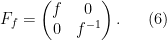
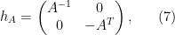
  . It is from these conditions that satisfy (3) that we often read in the literature the Lie algebra consisting of matrices of the form

 is an arbitrary matrix generating
  . Now, for anyone who has studied some double field theory, all of this will start looking familiar. Moreover, note that B is a two-form such that
  generates what we call B-transformations. In the context of generalised geometry,
  are
are  , with
  . In the maths literature,
 . Under this identification we therefore have

 . (What follows is a generalisation of the study of O(d,d) transformations on the level of the string spectrum. See, for instance, [Hitc10] and [Rub18]). The structure group
  generated by the following elements:
 Diffeomorphisms: It is important that from (
 we get for any
  the element
 . Although the connection may not be immediately obvious, we will see in a much later discussion in what way this transformation relates to diffeomorphisms on the target space. For now, observe that its action on
 on
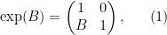
on  . Taking the exponential
 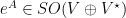 of (
of (
 we have an
  action

 matrix with integer entries. The two-form
  corresponding to the orthogonal transformation

 then acts

 but keeps V invariant. Similar to (
 is +1.
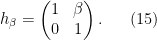
 and the 2-form
  in such a way that it is manifestly invariant under
  . When acting on the generalised metric, for the B-transformation we find

 with
with  a one-form on the worldsheet, these shifts are gauge transformations and they will be a topic of consideration in a later note.
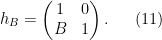
  these are transformations parametrised by an anti-symmetric
  matrix of the form
 is also +1. It gives the following action on

 on forms is defined by way of contraction. So, for some one-form
  it follows
  with
with  a local basis on the tangent space

 .
.
 and
and  , we can write the generalised vector
  , in which
  denotes the sections on E, in component form


 -invariant metric on the extended space (for the reader familiar with double field theory, this is indeed the
  on
on  and
and  on
on  over the patch
  as expected, where
  . For the index that runs over the entire extended space, it is conventional to use capital Latin letters
  . Hence,


 and
and  , there exists a natural canonical pairing between both sides of this direct sum

 so that the canonical orientation on E is defined by a real number.
![\displaystyle X_a = x_a + \xi_a = A^{-1}_{ab}x_b + [A^T_{ab} \xi_b - \iota_{A^{-1}_{ab} \alpha_b} B_{ab}], \ \ \ \ \ (27)](https://s0.wp.com/latex.php?latex=%5Cdisplaystyle++X_a+%3D+x_a+%2B+%5Cxi_a+%3D+A%5E%7B-1%7D_%7Bab%7Dx_b+%2B+%5BA%5ET_%7Bab%7D+%5Cxi_b+-+%5Ciota_%7BA%5E%7B-1%7D_%7Bab%7D+%5Calpha_b%7D+B_%7Bab%7D%5D%2C+%5C+%5C+%5C+%5C+%5C+%2827%29&bg=ffffff&fg=000000&s=0&c=20201002)
 suggest, we are considering the overlap of two local patches
  as an invertible matrix describing diffeomorphisms,
  a two-form, and
 is generated by elements denoted here as
  ,
,  such that, in the case of a triple overlap,
  the one-forms
  must satisfy

 , it is an element of
  . In the literature, this is interpreted to describe the structure of a gerbe, which at its most basic represents the analogue of a fibre bundle where the fibre is the classifying stack of a group. What it means is that
  , we will learn explicitly how the overall structure group
  and embeds as a subgroup of
  . This structure is actually quite interesting from the perspective of double field theory, but there is still much more to uncover before such considerations.
![\displaystyle [X, fY] = X(f)Y + f[X,Y]. \ \ \ \ \ (1)](https://s0.wp.com/latex.php?latex=%5Cdisplaystyle++%5BX%2C+fY%5D+%3D+X%28f%29Y+%2B+f%5BX%2CY%5D.+%5C+%5C+%5C+%5C+%5C+%281%29&bg=ffffff&fg=000000&s=0&c=20201002)

 with
with  and
and  .
.
 or
or  . This also takes us into a study of linear presymplectic and Poisson structures, but such preliminary discussion is dropped in these notes.
 , then for two generalised tangent vectors
 is purely convention with no geometric meaning.
  . Then the orthogonal compliment for this pairing can be defined in the standard sense

 is isotropic if
  . The idea of maximally isotropic subspaces raises interesting considerations, particularly globally defined structures with an integrability condition, which are often studied under the heading of linear Dirac structures. As a matter of introduction, if
  for
for  for
for  as the total basis for
  with the canonical pairing given by
 . In fact, this statement is true for any maximally isotropic subspace.
 .
.
 to be semidefinite such that
  or
or  for all
  . Otherwise, consider a compliment
  so that
  , then if
  with
with  and
and  , a suitable linear combination
  would be null. As a result
  would be isotropic containing
  we have

 such that we now have
 so
so  .
.  with a symmetric pairing of signature
  given by


 is denoted Cliff(E).


 are vector parts and
  1-form parts.
The set of smooth sections
1-form parts.
The set of smooth sections  of the bundle
  and the set of smooth 1-forms by
  .
Remark 4 (Sequence and string background fields) For the sequence (
.
Remark 4 (Sequence and string background fields) For the sequence ( there exist sections
  that are given by rank 2 tensors, which can then be split into symmetric and antisymmetric parts,
  . The sections of

You must be logged in to post a comment.