Tao’s smoothed asymptotics

On February 8, 2024February 16, 2024 By Robert G. C. SmithIn Mathematics, Physics

In a recent paper, we explored possible connections between analytic number theory and the study of divergent series and the ultra-violet regularisation of loop integrals in perturbative quantum field theory. This project started quite innocently but eventually turned into a research programme that we’re really quite excited about, with many more interesting results and connections to be reported in our second paper and beyond. On the number theory side, an early motivation for our work was an expository article on smoothed asymptotics by Terence Tao. This article was first published on his blog; it was also included in his book Compactness and Contradiction, which is a collection of loosely related articles that explore the connections between finitary and infinitary mathematics. I personally prefer not to view his exposition on smoothed asymptotics in isolation of the book, because, although somewhat blurry, I sometimes think that maybe there is more to do with Tao’s definition of a compactness and contradiction argument from a physicist’s point of view, not least in relation to our ongoing work but also more generally in terms of the idea of constructing a bridge between the finitary (or quantitative) and the infinitary (or qualitative). But this is speculative, and I do not want to distract.

In this post, I’ll review some basics of Tao’s smoothed asymptotics and also make one or two comments about our paper.

Consider the sums of powers written in terms of their discrete partial sums:

$\displaystyle 1 + 2 + 3 + ... + n = \frac{1}{2}n(n+1) = \frac{1}{2}n + \frac{1}{2}n^2, \ \ \ \ \ (1)$

$\displaystyle 1^2 + 2^2 + 3^2 + ... + n^2 = \frac{1}{6}n(n+1)(2n + 1) = \frac{1}{6} n + \frac{1}{2}n^2 + \frac{1}{3}n^3, \ \ \ \ \ (2)$

$\displaystyle 1^3 + 2^3 + 3^3 + ... + n^3 = \frac{1}{4}n^2(n+1)^2 = \frac{1}{4}n^2 + \frac{1}{2}n^3 + \frac{1}{4}n^4. \ \ \ \ \ (3)$

These three discrete sums (1–3), which have been represented as closed formulae, can be written as the general sum of powers ${\sum \limits_{n=1}^k n^i}$ with ${i}$ a fixed integer. When thought of in this way, we can compare the partial sums with their corresponding (infinite) divergent series. I will also include the case for ${i=0}$ :

$\displaystyle 1 + 1 + 1 + 1 + \dots = \sum \limits_{n=1}^{\infty} n^0, \ \ \ \ \ (4)$

$\displaystyle 1 + 2 + 3 + 4 + \dots = \sum \limits_{n=1}^{\infty} n, \ \ \ \ \ (5)$

$\displaystyle 1^2 + 2^2 + 3^2 + 4^2 + \dots = \sum \limits_{n=1}^{\infty} n^2, \ \ \ \ \ (6)$

$\displaystyle 1^3 + 2^3 + 3^3 + 4^3 + \dots = \sum \limits_{n=1}^{\infty} n^3. \ \ \ \ \ (7)$

As mentioned in our recent paper in relation to these formulae: the primary issue with such divergent series appears in the transition from partial sums to infinity. This was most notably exposed by Ramanujan, and is made explicit in the use of Tao’s methodology.

The easiest way to see this issue is to note that the formulae (1–3) are special cases of Faulhaber’s formula

$\displaystyle \sum_{n=1}^N n^z=\frac{1}{z+1} \sum_{n=0}^z \binom{z+1}{n} B_n N^{z-n+1}, \ \ \ \ \ (8)$

where ${z}$ is a positive integer and ${B_n}$ are the Bernoulli numbers (we follow the convention ${B_1= 1/2}$ ). In the limit ${N \rightarrow \infty}$ Faulhaber’s formula breaks down.

On the other hand, we know that we can compute the divergent series (4–7) using the Riemann zeta function. The Riemann zeta function ${\zeta(s)}$ is defined in the region ${Re(s) > 1}$ by the absolutely convergent series

$\displaystyle \zeta(s) = \sum \limits_{n=1}^{\infty} \frac{1}{n^s} = 1 + \frac{1}{2^s} + \frac{1}{3^s} + \dots. \ \ \ \ \ (9)$

After analytic continuation one has for the sums of powers ${\zeta(0) = -1/2}$ , ${\zeta(-1) = -1/12}$ , and so on, so that in general we can define a direct relation with the Bernoulli numbers

$\displaystyle \zeta(-s) = -\frac{B_{s+1}}{s+1}. \ \ \ \ \ (10)$

And so, if one formally applies (9) we obtain

$\displaystyle \sum \limits_{n=1}^{\infty} n^0 = 1 + 1 + 1 + \dots = -1/2, \ \ \ \ \ (11)$

$\displaystyle \sum \limits_{n=1}^{\infty} n = 1 + 2 + 3 + \dots = -1/12, \ \ \ \ \ (12)$

$\displaystyle \sum \limits_{n=1}^{\infty} n^2 = 1 + 4 + 9 + \dots = 0, \ \ \ \ \ (13)$

and so on for each integer value ${i}$ in the sum ${n^i}$ , which evidences the general pattern

$\displaystyle \sum \limits_{n=1}^{\infty} n^s = 1 + 2^s + 3^s + \dots = -\frac{B_{s+1}}{s+1}. \ \ \ \ \ (14)$

What we obtain therefore is a collection of bizarre, if not altogether absurd, formulae. In the classical sense of summation they do not appear in any way coherent or reasonable, with one obvious reason being that we have positive summands appearing to equate to some negative or zero value.

As Tao clearly demonstrates in his article, if one tries to inspect the partial sums of these divergent series there is no obvious relationship with the constant values appearing in (11–13). From Faulhaber’s formula, if we apply it to (14) we obtain

$\displaystyle S_s(N) = \sum \limits^N_{n=1} n^s = \frac{1}{s+1}N^{s+1} + \frac{1}{2}N^s + \frac{s}{12}N^{s-1} + ... + B_s N, \ \ \ \ \ (15)$

which resembles very little of the right-hand side of the formulae (11–13). One of the main issues here has to do with the discrete nature of the partial sum, particularly in the transition to infinite series. When one uses partial sums to sum an infinite series ${\sum \limits_{n=1}^{\infty} a_n}$ , one is imposing a sharp truncation of that series at some finite ${N}$ . So what one is really doing is modifying the infinite series with a step function such that for ${f : \mathbb{R} \rightarrow \mathbb{R}}$ it can be written

$\displaystyle f(x) = \sum \limits_{n=1}^{\infty} a_n \theta \left(\frac{n}{N}\right) = \sum \limits_{n=1}^{N} a_n, \ \ \ \ \ (16)$

where

$\displaystyle \theta(x)=\begin{cases} 1 & x \leq 1 \\ 0 &x>1 \end{cases}. \ \ \ \ \ (17)$

For example, consider the divergent series (4). When looking at the ordinary partial sums and plotting them as a function of ${N}$ one will obtain a step graph, in which there exist jump discontinuities at integer values ${N}$ (for example, see this Wiki).

From a physics point of view, I think there is reasonable grounds to ask why this should be considered the most natural way to treat infinite (divergent) series. There are physical examples we might draw on to ask, why not a smooth cutoff instead?

Perhaps an example of Tao’s notion of post-rigour, by which it is meant that from the foundations of mathematical rigour one may allow the guidance of good intuition, I see the idea of smoothed asymptotics as creating a conceptual bridge of sorts. Instead of considering the ill-behaved discrete series ${\sum \limits_{n=1}^N a_n}$ , it can be replaced so that the convergence of a series is defined through the limit

$\displaystyle \lim \limits_{N \rightarrow \infty} \sum \limits_{n=1}^{\infty} a_n \eta \left(\frac{n}{N}\right), \ \ \ \ \ (18)$

where ${\eta : [0, \infty) \rightarrow \mathbb{R}}$ equals the characteristic function of the interval ${[0,1]}$ . As a bounded function of compact support, we shall call any ${\eta}$ a cutoff function satisfying the conditions

$\displaystyle \eta(x)=\begin{cases} 1 & x \in [0,1] \\ 0 &x>1 \end{cases}. \ \ \ \ \ (19)$

One can ask if it is possible to consider other possible cutoffs ${\eta}$ , and, indeed, this is precisely what we do. In fact, we find that ${\eta}$ can be any Schwartz function so long that the smooth cutoff is normalised to ${\eta(0) = 1}$ . (It is also possible, as Tao notes, that the assumption of compact support in the interval ${[0,1]}$ can be extended to a more general case, which can be deduced by redefining the ${N}$ parameter). We show therefore that in extending Tao’s methodology we can define an infinite class of smooth cutoff functions ${\eta}$ , and a lot of time has since been spent studying what might be described as special subclasses of such cutoff functions!

The method of smooth asymptotics also has a lovely relation with the Euler-Maclaurin formula, which, for me, is one of the most beautiful formulae in modern mathematics. This was beautifully elucidated by Tao. We see that the Euler-Maclaurin formula gives a lot of information that helps one understand the results of smoothed asymptotic expansions, and also serves to define a rather lovely relation between smoothed sums and the Riemann zeta function (I will discuss much of this in another post, because I want to build the picture first from a derivation of the E-M formula as I think this gives some nice intuition about smoothed sums). We can also prove a lot of nice properties about ${\eta}$ without the Euler-Maclaurin formula, using many of the basic tools from analysis. For instance, earlier I mentioned convergence of smoothed sums. Recall the definition of series convergence:

$\displaystyle \sum \limits_{n=1}^{\infty} a_n = s \ \text{iff} \ \lim \limits_{N \rightarrow \infty} \sum \limits_{n=1}^{N} a_n = s \ \ \ \ \ (20)$

with ${s \in \mathbb{R}}$ . In the language of smoothed sums, we can equivalently define convergence of series as

$\displaystyle \lim \limits_{N \rightarrow \infty} \sum \limits_{n=1}^{\infty} a_n \left(\frac{n}{N}\right). \ \ \ \ \ (21)$

A convergent series ${\sum a_n}$ of non-negative terms is absolutely convergent, since ${\sum a_n}$ and ${\lvert \sum a_n \rvert}$ are the same. Using the fact that ${\eta}$ is bounded, since there is an ${M > 0}$ such that ${\mid \eta(x) \mid < M}$ for all ${x}$ , and the fact that ${\eta}$ is continuous, one can show that for the absolutely convergent sum ${\sum \limits_{n=1}^{\infty} a_n}$ it also true ${\lim \limits_{N \rightarrow \infty} \sum \limits_{n=1}^{\infty} a_n \eta \left(\frac{n}{N}\right) = s}$ . One can similarly prove the case where ${\sum \limits_{n=1}^{\infty}a_n}$ is conditionally convergent.

***

From a physics perspective, this general idea of using a smooth cutoff function is not necessarily new. Often when dealing with divergent integrals in QFT, one approach is to introduce some sort of function to smear or smooth interactions. This can be thought of formally in the space of distributions. In a more direct and physically intuitive manner, a textbook example is how one might simply consider in place of a sharp momentum cutoff some smooth cutoff function ${\rho(p, \Lambda)}$ in Euclidean space. This smooth cutoff is then defined such that ${\lim_{p \rightarrow \infty} \rho(p, \Lambda) = 0}$ when ${\lambda}$ is fixed. Or, when ${p}$ is fixed, ${\lim_{\Lambda \rightarrow \infty} \rho(p, \Lambda) = 1}$ . An example of an explicit choice of cutoff is ${\rho = \exp(-p^2 / \Lambda^2)}$ . Another intuitive example from physics can be found in Joe Polchinski’s great work on renormalisation group flow equations, where a simple smooth regulator function is introduced. Similarly, in the heat-kernel approach to QFT and its rigorous mathematical formulation, one finds motivation for the use of a smooth cutoff function. In more general scenarios, such as quantum gravity, the reluctance of string theory to travel deep into the UV is a direct manifestation of the smoothing or smearing effect of the string length scale (as seen in a study of modular invariance of the worldsheet).

Perhaps one of the oldest examples, as referenced in Matthew D. Schwartz’s wonderful textbook on QFT and the standard model, comes from the calculation of the Casimir effect. In his original paper, Casimir showed that there is a way to calculate the force in a regulator independent way. In this approach the energy is defined as

$\displaystyle E(a) = \frac{\pi}{2} \sum \limits_n \frac{n}{a} f \left( \frac{n}{a\Lambda} \right), \ \ \ \ \ (22)$

where ${f(x)}$ is a generic cutoff function. It is shown that any sensible regulator will correctly give the Casimir force so long that ${\lim \limits_{x \rightarrow \infty} xf^{(i)}(x) = 0}$ and at the origin ${f(0) = 1}$ . In taking this approach it is possible to choose as a special case any one of the common regularisation schemes that satisfies the above conditions.

This raises the question whether there is a more general way to formulate such an idea for all QFTs. We show that $\eta$ regularisation is, indeed, incredibly general in the extended setting. In fact, in the context of perturbative QFT we can capture all of the common regularisation schemes as a particular choice of $\eta$ . What’s more, both Tao’s methodology and QFT exhibit regulator dependence of power law divergences, while the universal features of finite terms in Tao’s study of divergent series mirror conjectured universal features of logarithms in QFT. These are among a number of insights that provide intriguing hints at potentially something deeper. But most fascinatingly, we also found a surprising connection between the ${\eta}$ regularisation of divergent series in analytic number theory and the preservation of gauge invariance at one loop in a regularised quantum field theory! This result is the main feature of our first paper. We show in the calculation of the vacuum polarisation that cancellation of the quadratic divergences requires precisely enhanced regulators of order one, which goes back to the fact that for sum of the naturals the corresponding Mellin transform is vanishing $C[\eta]=0$ . It is really quite a beautiful result.

Theorem connecting partial sums and the values of the Riemann zeta function

On January 15, 2024January 18, 2024 By Robert G. C. SmithIn Mathematics

In the course of some studies relating to our first paper on analytic number theoretic sums and quantum field theory, I came across a simple yet seemingly not too well known theorem (as far as I have seen in the literature; however I do note the likeness to, and manner from which the result can be directly extrapolated from, Hans Rademacher’s 1973 book Topics in Analytic Number Theory). The theorem can be found in a short paper by Jan Minac from 1994. The main result gives a slightly different perspective on the relation between the values of the Riemann zeta function and the partial sums of the sums of integer powers.

The origin of the Riemann zeta function ${\zeta(s)}$ goes back to the study of many-particle systems and how they may be encoded in a single partition function. In 1737, Euler proved the identity

$\displaystyle \prod \limits_p (1 - \frac{1}{p^s})^{-1} = \sum \limits_{n=1}^{\infty} = \zeta(s), \ \ \ \ \ (1)$

which holds for all real numbers ${s > 1}$ and, amazingly, refers to all prime numbers ${p}$ . After Euler’s introduction of ${\zeta (s)}$ over the real numbers, it was Bernhard Riemann in his seminal 1859 paper who took this formula as his starting point and extended it to a complex variable. In the process, he proved among other things the relation between its zeros and the distribution of prime numbers. From this comes the Riemann zeta function, which can be written as the sum of the reciprocals of the positive integers

$\displaystyle \zeta(s)=\sum \limits_{n=1}^{\infty}\frac{1}{n^{s}}=1+\frac{1}{2^s}+\frac{1}{3^s}+ \dots, \ \ \ \ \ (2)$

where ${s}$ is a complex number with ${Re(s) > 1}$ . For negative integers (and also zero), the Riemann zeta function can be related to the Bernoulli numbers ${\zeta(-s) = (-1)^s B_{s+1} / (s+1)}$ . Another remarkable fact about this, and about the Bernoulli numbers in general, is that all the values ${\zeta(-s)}$ are rational numbers: ${\zeta(-1) = - 1/12}$ , ${\zeta(-2) = 0}$ , ${\zeta(-3) = 1/120}$ , and so on.

From the definition of Faulhaber’s formula, heuristically there is a relation ${\sum \limits_{n=1}^{\infty} n^s = \frac{(-1)^s B_{s+1}}{s+1}}$ that can be deduced, which agrees with the value of the Riemann zeta function for negative integers ${s = -p >0}$ . However, in general, when one expands the partial sums for the respective sums of integer powers, there is no obvious relationship between the partial sum form and the values obtained by the zeta function as indicated in the above equality.

Interestingly, from Minac’s paper, we see that we can define the partial sums ${S_a (N) := \sum \limits_{n=1}^{N-1} n^a}$ such that they are expressible as polynomials in ${N}$ of degree ${a+1}$ with rational coefficients (again, see Rademacher’s 1973 book). One can then ask whether any connection between ${\zeta(-a)}$ and ${S_a(N)}$ can be made. This leads us to the main theorem of Minac’s paper, for which I also repeat the proof.

Theorem 1 : Consider the power sum ${S_a (N) = \sum \limits_{n=1}^{N-1} n^a}$ . For positive integers ${a}$ there exists the relation ${\zeta(-a) = \int_0^1 dx \ S_a (x)}$ .

Proof: Let ${B_k}$ be the kth Bernoulli number for ${k = 0,1,2,\dots}$ , and ${B_0(x) = 1}$ . For each ${m \in \mathbb{N}}$ we define the mth Bernoulli polynomial ${B_m (x) = \sum \limits_{k=0}^{m} \begin{pmatrix} m \\ k \\ \end{pmatrix} B_k x^{m-k}}$ . Importantly, we note ${B_m(1) = (-1)^m B_m = (-1)^m B_m(0)}$ , and the derivative of the Bernoulli polynomial takes the form ${d/dx \ B_m (x) = mB_{m-1}(x)}$ . Finally, we shall use the fact ${S_a(N) = \frac{B_{a+1}(N) - B_{a+1}(1)}{a+1}}$ , which is based on one of the most important properties of Bernoulli polynomials $B_m (x + 1) - B_m (x) = mx^{m-1}$ , as well as ${\zeta(-a) = (-1)^a \frac{B_{a+1}}{a+1} = - \frac{B_{a+1}}{a+1}}$ for ${a \in \mathbb{N}}$ .

Since ${S_a(N)}$ is polynomial in ${N}$ of degree ${a + 1}$ , the important observation is that we can exploit these basic properties of Bernoulli polynomials to establish the integration of the polynomial representation ${S_a(N)}$ of the partial sums from ${0}$ to ${1}$ . Let ${a \in \mathbb{N}}$ , then from the above it follows

$\displaystyle \int_0^1 dx \ S_a(x) = \int_0^1 \frac{B_{a+1}(x) - B_{a+1}(1)}{a+1}$

$\displaystyle = \frac{B_{a+2}(1) - B_{a+2}(0)}{(a+1)(a+2)} + (-1)^a \frac{B_{a+1}}{a+1} = 0 + (-1)^a \frac{B_{a+1}}{a+1} = \zeta(-a). \ \ \ \ \ (3)$

$\Box$

As an example, let us consider one of my favourite cases: the sum of natural numbers corresponding formally to ${zeta(-1)}$ . Theorem 1 gives

$\displaystyle 1 + 2 + 3 + 4 + \dots = \zeta(-1) = \int_0^1 dx \ \frac{x(x - 1)}{2}= \int_0^1 dx \ \left(\frac{x^2}{2} - \frac{x}{2}\right) = \frac{1}{6} - \frac{1}{4} = -\frac{1}{12}. \ \ \ \ \ (4)$

Very cool!

[1] Ján Mináč, “A remark on the values of the Riemann zeta function,” Expositiones Mathematicae, 12: 459-462, 1994.

Bernoulli numbers

On October 3, 2023December 11, 2023 By Robert G. C. SmithIn Mathematics

“Of the various special kinds of numbers used in analysis, there is hardly a species that is so important and so generally applicable as the Bernoulli Numbers. Their numerous properties and applications have caused the creation of an extensive literature on the subject which still continues to attract the attention of scholars.” [1]

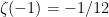
Let’s go back to the sum of integer powers $1^s + 2^s + \dots + n^s$ for a moment. The sum of the sth power $n^s$ of the first positive integers $k$ is given by a polynomial in $n$ :

$\displaystyle S_s(n):= 1^s + 2^s + \dots + n^s = \sum \limits_{k=1}^{\infty} k^s. \ \ (1)$

We know the first form of the Bernoulli formula, at least in terms of modern notation, can be written in terms of combinatorial factors

$\displaystyle S_s(n) = \frac{1}{s + 1}\bigg\{\begin{pmatrix} s+1 \\ 0 \\ \end{pmatrix}\sigma^0_1 n^{s+1} + \begin{pmatrix} s + 1 \\ 1 \end{pmatrix} \sigma_1^1 n^s + \begin{pmatrix} s+1 \\ 2 \\ \end{pmatrix}\sigma^2_1 n^{s-1} + \dots + \begin{pmatrix} s+1 \\ s \\ \end{pmatrix} \sigma^s_1 n \bigg\}, \ \ (2)$

where $\sigma_m^s$ for $m=1$ denote the coefficients of the expansion. In \textit{Ars Conjectandi}, Bernoulli calculated the formulas for $S_s(n)$ up to ten using the methods of Fermat. If we were to study the structure and pattern of these coefficients $\sigma^s_m$ we would find a well-known table for the first six sums up to $s-1$

Notice there is indeed a really nice pattern. The coefficient of $n^{s+1}$ in $S_s(n)$ is always $1/(s+1)$ . The coefficient of $n^s$ is always $1/2$ . The coefficient of $n^{s-1}$ is always $s/12$ , and so on.

This is more or less the origin story of the Bernoulli numbers. That is, when we study the recurrence relations associated with the formula (\ref{Bernoulliformula}) we find for fixed coefficients $\sigma^s_1$ the Bernoulli numbers $B_n$ (ignoring discrepancies of (-1)). We may write them explicitly in place of the coefficients $\sigma_1^m$ so that

$\displaystyle \sum \limits_{k=1}^{n} k^s = \frac{1}{s+1}\bigg \{B_0 n^{s+1} - \begin{pmatrix} s+1 \\ 1 \\ \end{pmatrix} B_1 n^s + \begin{pmatrix} s+2 \\ 2 \end{pmatrix} B_2 n^{s-1} +...+ (-)^s \begin{pmatrix} s+1 \\ k \\ \end{pmatrix} B_s n \bigg \}. \ \ (3)$

We can rewrite this more compactly in terms of the very nice and famous formula

$\displaystyle \sum \limits_{k=1}^{n} k^s = \frac{1}{s+1}\sum \limits_{k=0}^{s}\begin{pmatrix} s+1 \\ k \end{pmatrix}B_k n^{s+1 - k}, \ \ (4)$

which in some literature is called Bernoulli’s formula, and if I remember correctly it is given in his work Summae Potestatum, albeit not quite like this. Alternatively, one might also call it Faulhaber’s formula. Faulhaber discovered it independently without knowing of the existence of the Bernoulli numbers $B_k$ . One can see that the Bernoulli numbers are defined here in terms of the recursion relation $\sum \limits_{k=0}^{n} \begin{pmatrix} s+1 \\ k \end{pmatrix}B_k = s+1$ . Equivalently, and perhaps most famously, they may also be defined in terms of the generating function

$\displaystyle \frac{z}{1 - e^{-z}} = \sum \limits_{k=0}^{\infty} B_k \frac{z^k}{k!}.$

To give some examples, notice $\sigma_1^0 = B_0 = 1$ , with the dominant term (of $s+1$ in $n$ ) always $\frac{1}{s+1}n^{s+1}$ (which, interestingly, coincides with the integral $\int_0^n x^s dx$ . It evokes the question in what way the sum of integer powers, and perhaps the Bernoulli numbers, know of a deeper relation between discrete sums and continuous integrals. But I’ll save this for another time). If $s=0$ , we recover

$\displaystyle \sum \limits_{k=1}^n k^0 = \sum \limits_{k=1}^n 1 = n. \ \ (5)$

If $s=1$ , then we recover the next partial sum (triangular numbers)

$\displaystyle \sum \limits_{k=1}^n k = \frac{n(n+1)}{2}, \ \ (6)$

and for $s=2$ we obtain the square pyramidal numbers

$\displaystyle \sum \limits_{k=1}^n k^2 =\frac{n(n+1)n(2n+1)}{6}, \ \ (7)$

and so on. From another point of view, the partial sums for the sums of integer powers are a special case of the formula (4). The small Bernoulli numbers are given below

$\displaystyle B_0 = 1, B_1 = \frac{1}{2}, B_2 = \frac{1}{6}, B_4 = -\frac{1}{30}, B_6 = \frac{1}{42},..., \ \ (8)$

using the convention that $B_1 = 1/2$ .

What’s really interesting about the Bernoulli numbers is how they are ubiquitous throughout maths and physics. They show up almost everywhere, not only in number and analysis but in the expansions of trigonometric functions, quantum field theory and string theory, to name a few. They also play an important role in the Euler-Maclaurin summation Formula, the evaluation of the Riemann zeta function, and in Fermat’s Last Theorem. Yet there is currently no universal theory (that I am aware of) explaining their appearance in many different contexts. In many ways, Euler started the journey in trying to better understand the Bernoulli numbers, using them to derive a solution to the even values of the zeta function. But even Euler couldn’t completely capture these numbers. Despite their mystery, we can learn a bit about these numbers through the Euler-Maclaurin formula, beginning with a derivation from the view of discrete calculus.

[1] David Eugene Smith. A Source Book in Mathematics, McGraw-Hill, N.Y., 1929.

TracingCurves

Tag: Sums of Powers

Tao’s smoothed asymptotics

Theorem connecting partial sums and the values of the Riemann zeta function

Bernoulli numbers